This page outlines the key formulae, principles, and concepts forming the mathematical foundations of AC metrology used within LMA.
Context
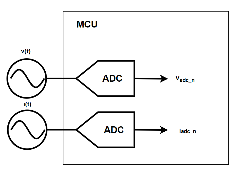
In metrology, measurements begin at the raw ADC level, where we acquire discretised instantaneous samples of both voltage and current.
Thus, we have: \( v(t) \) and \( i(t) \)
Specifically in the form of ADC samples: \( V_\mathrm{adc_n} \) & \( I_\mathrm{adc_n} \)
These represent the instantaneous voltage and current waveforms.
All subsequent calculations—RMS, power, and energy—are derived directly from these sampled signals.
RMS
When analysing AC systems, we are often interested in average quantities.
However, since the average of a pure sine wave over one period is zero, using a simple mean would yield no useful measurement of power or energy.
Instead, we use the Root Mean Square (RMS), which represents an AC systems equivalent DC value.
Mathematically:
\[x_\mathrm{RMS} = \sqrt{ \frac{1}{N} \sum_{n=1}^{N} x_n^2 } \]
This concept forms the foundation of AC metrology.
Voltage
Using the instantaneous voltage signal \( v(t) \), the RMS value is:
\[V_\mathrm{RMS} = \sqrt{ \frac{1}{T} \int_0^T [v(t)^2] \, dt } \]
In discrete digital form (using ADC samples):
\[V_\mathrm{RMS} = \sqrt{ \frac{1}{N} \sum_{n=1}^{N} [V_\mathrm{adc_n}^2] } \]
Where:
- \( N \) = number of samples
- \( V_\mathrm{adc_n} \) = voltage sample
Current
Similarly, for current:
\[I_\mathrm{RMS} = \sqrt{ \frac{1}{T} \int_0^T [i(t)^2] \, dt } \]
Discrete form:
\[I_\mathrm{RMS} = \sqrt{ \frac{1}{N} \sum_{n=1}^{N} [I_\mathrm{adc_n}^2] } \]
Where:
- \( N \) = number of samples
- \( I_\mathrm{adc_n} \) = current sample
Frequency
In AC systems, frequency refers to the fundamental line frequency, typically 50 Hz or 60 Hz depending on the region.
Accurate frequency measurement is crucial for power computation, phase determination, and system diagnostics.
A common digital approach is to first filter the voltage signal to isolate the fundamental component and remove high-frequency noise or harmonics, then perform zero-crossing detection on the filtered waveform.
Zero-crossing detection identifies points where the voltage waveform passes through zero in a defined direction (negative-to-positive or positive-to-negative), which serve as time markers of the AC cycle.
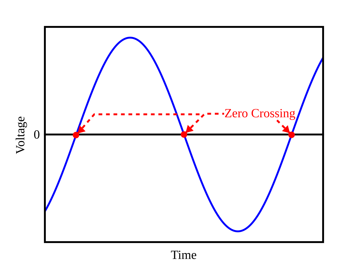
In a digital system, the voltage signal is represented by discrete ADC samples, \( V_\mathrm{adc_n} \), where \( n \) indexes the sample.
A zero crossing occurs between samples \( V_\mathrm{adc_n} \) and \( V_\mathrm{adc_{n+1}} \) where the sign of the voltage changes.
The frequency can then be calculated as:
\[f = \frac{1}{N \cdot \delta_t} [Hz] \]
Where:
- \( N \) = number of ADC samples between consecutive zero crossings of the same polarity
- \( \delta_t \) = sampling interval (seconds)
- \( V_\mathrm{adc_n} \) = voltage ADC sample at index \( n \)
Power
Power in AC systems is derived directly from voltage and current waveforms defined as:
\[v(t) = V_\mathrm{m} \sin(2 \pi f t) \]
\[i(t) = I_\mathrm{m} \sin(2 \pi f t) \]
Where:
- \( V_\mathrm{m} \) = peak voltage
- \( I_\mathrm{m} \) = peak current
- \( f \) = line frequency
- \( t \) = time
Phase Shift
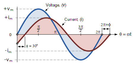
An important topic to cover before going into power computations however is the phase relationship of current and voltage.
Current and voltage are often out of phase due to reactive components (inductors or capacitors).
The angular displacement between them is the phase shift, \( \phi \), a key parameter for determining active and reactive power.
This means we must modify our voltage and current signals to better represent the system:
\[v(t) = V_\mathrm{m} \sin(2 \pi f t) \]
\[i(t) = I_\mathrm{m} \sin(2 \pi f t + \phi) \]
Where \( \phi \) denotes the phase angle:
- Positive ( \( \phi > 0 \)): current leads voltage (capacitive load)
- Negative ( \( \phi < 0 \)): current lags voltage (inductive load)
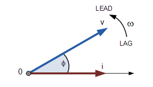
This is often nicely shown in the form of a phasor diagram.
Apparent Power
Apparent power \( S \), measured in \( VoltAmperes [VA] \), represents the total system power (both useful and reactive components):
\[S = V_\mathrm{RMS} I_\mathrm{RMS} \]
Discrete form:
\[S = \frac{1}{N} \sqrt{ \sum_{n=1}^{N} [V_\mathrm{adc_n}^2] \cdot \sum_{n=1}^{N} [I_\mathrm{adc_n}^2] } \]
Active Power
Active (real) power \( P \), measured in \( Watts [W] \), is the component that performs useful (resistive) work:
\[P = \frac{1}{T} \int_0^T [v(t) i(t)] dt \]
Discrete form:
\[P = \frac{1}{N} \sum_{n=1}^{N} [V_\mathrm{adc_n} I_\mathrm{adc_n}] \]
Reactive Power
Reactive (imaginary) power \( Q \), measured in \( VoltAmperesReactive [VAR] \), is the component that performs no net work in the system.
It represents energy exchanged with inductive or capacitive components.
We can understand reactive power by recalling three key points about phase relationships:
- A purely resistive load has 0° phase shift between voltage and current.
- A purely reactive load has a 90° phase shift between voltage and current.
- Instantaneous active power is always given by \( p(t) = v(t) \cdot i(t) \).
From this, we can derive an important concept, if we artificially shift the current waveform by 90°, the resulting active power becomes zero, leaving only the reactive component.
Therefore mathematically introducing a 90° shift in current gives:
\[ q(t) = v(t) \cdot i(t - 90^\circ) = V_\mathrm{pk} \sin(2 \pi f t) \cdot I_\mathrm{pk} \sin(2 \pi f t + \phi - 90^\circ) \]
Discrete form:
\[ Q = \frac{1}{N} \sum_{n=1}^{N} [V_\mathrm{adc_n} \cdot I_\mathrm{adc_n-90^\circ}] \]
Where:
- \( V_\mathrm{adc_n} \) = voltage sample at index \( n \)
- \( I_\mathrm{adc_n-90^\circ} \) = current sample phase-shifted by 90°
Return to Phase Shift
Using the relationship between active, reactive and apparent power we can start to exploit this for extracting more important information. Metering systems are far from ideal, they contain filters with components of varying tolerance, PCB's with mismatched traces and potential noise soruces non-uniformly impacting the signals. This leads to a common problem that even when monitoring a purely active load (UPF or Unity Power Factor) there may "look like" there is still a phase shift due to errors in our sampling chain.
However we can calibrate this out - lets say we take our current voltage and votlage shifted samples and compute active and reactive powers. But if we know the load to be purely active, we know the reactive component is due entirely to erroneous phase shift. So we can use the relationship between active and reactive power in the power triangle to derive the phase error:
\[\theta = \tan^{-1}\left(\frac{Q}{P}\right) \cdot \frac{180}{\pi} \]
Where:
- \( \theta \) = Phase Error in degrees
- \( Q \) = Reactive power
- \( P \) = Active power
We can use this to perform phase compensation in our signal chain to "realign" the signals - this is common practise and often a necessary requirement for achieving suitable accuracy standards.
Power Factor (PF)
The Power Factor (PF) expresses how efficiently power is used and is defined as:
\[\mathrm{PF} = \cos(\phi) \]
Thus:
- Purely Resistive: \( \phi = 0^\circ \Rightarrow \mathrm{PF} = 1 \)
- Purely Reactive: \( |\phi| = 90^\circ \Rightarrow \mathrm{PF} = 0 \)
- Mixed Load: \( 0 < |\phi| < 90^\circ \Rightarrow 0 < \mathrm{PF} < 1 \)
The easiest way to compute the power factor is using apparent and active power:
\[\mathrm{PF} = \cos(\phi) = \frac{S}{P} \]
Energy
Energy is the cumulative measure of total work done or power consumed by a system over time.
In AC metrology, we do not compute energy directly from voltage and current samples; instead, we build on previously defined power computations.
Energy computation flow:
- Compute average power ( \( P, Q, S \)) over a defined measurement period.
- Derive the corresponding energy for that period.
- Accumulate these periodic energy values over time to obtain total energy consumption.
Instantaneous power is defined as:
\[ p(t) = v(t) \cdot i(t) \]
And energy is the integral of power over time:
\[ E = \int_0^T p(t) \, dt \]
In a discrete digital system, we process data in finite computation windows of samples ( \( N \)).
This means energy per unit time becomes:
\[ E = P \cdot \delta \]
In a system with a fixed sampling period \( \delta \) becomes \( \frac{1}{f_s} \) and an energy quanta per sampling period can be defined:
\[ E_\mathrm{unit} = \frac{P}{f_s} \]
Where:
- \( P \) = Computed average power.
- \( f_s \) = System sampling frequency.
- \( E_\mathrm{unit} \) = Energy quanta per ADC sample.
And we can use this quanta by incrementing a running total of energy every time a sampling period passes:
\[ E_\mathrm{t} = E_\mathrm{t,prev} + E_\mathrm{unit} \]
Where:
- \( E_\mathrm{t} \) = Current running total of energy.
- \( E_\mathrm{t,prev} \) = Previous (before increment) running total of energy.
The table below summarises the computation of energy per sampling period (unit) and accumulated totals for active, reactive, and apparent power.
| Type | Instantaneous Power | Average Power | Energy Unit | Accumulated Energy Total | Units |
|---|---|---|---|---|---|
| Active | \( p(t) = v(t) \cdot i(t) \) | \( P = \frac{1}{N} \sum_{n=1}^{N} [V_\mathrm{adc_n} \cdot I_\mathrm{adc_n}] \) | \( E_\mathrm{active,unit} = \frac{P}{f_s} \) | \( E_\mathrm{active,t} = E_\mathrm{active,t,prev} + E_\mathrm{active,unit} \) | Ws |
| Reactive | \( q(t) = v(t) \cdot i(t - 90^\circ) \) | \( Q = \frac{1}{N} \sum_{n=1}^{N} [V_\mathrm{adc_n} \cdot I_\mathrm{adc_n-90^\circ}] \) | \( E_\mathrm{reactive,unit} = \frac{Q}{f_s} \) | \( E_\mathrm{reactive,t} = E_\mathrm{reactive,t,prev} + E_\mathrm{reactive,unit} \) | VARs |
| Apparent | Not Applicable | \( S = \frac{1}{N} \sqrt{\sum_{n=1}^{N} V_\mathrm{adc_n}^2 \cdot \sum_{n=1}^{N} I_\mathrm{adc_n}^2} \) | \( E_\mathrm{apparent,unit} = \frac{S}{f_s} \) | \( E_\mathrm{apparent,t} = E_\mathrm{apparent,t,prev} + E_\mathrm{apparent,unit} \) | VAs |
Where:
- \( N \) = number of samples per computation window
- \( f_s \) = sampling frequency
This table provides a compact overview of how each type of energy is calculated per computation window and accumulated over time, including their respective units.
Where:
- \( E_\mathrm{active,t} \) is in watt-seconds [Ws]
- \( E_\mathrm{reactive,t} \) in volt-ampere reactive seconds [VARs]
- \( E_\mathrm{apparent,t} \) in volt-ampere seconds [VAs]
To summarise, energy accumulation follows this loop:
- Collect \( N \) ADC samples for voltage and current.
- Compute average powers \( P, Q, S \) for the computation window.
- Convert each power to energy quanta \( E_\mathrm{unit} = \frac{P}{f_s} \).
- Accumulate totals for active, reactive, and apparent energy.
- Periodically store totals in non-volatile memory to preserve state.
Harmonics
- Todo
- Describe harmonic analysis, distortion, and total harmonic distortion (THD)
Filtering
Filtering is an essential part of digital metrology, removing DC bias, noise, and high-frequency components.
HPF
A High-Pass Filter (HPF) attenuates low frequencies (including DC). Its cutoff frequency, \( f_c \), defines where attenuation begins (–3 dB point).
\[y_n = \alpha y_{n-1} + \alpha (x_n - x_{n-1}) \]
\[\alpha = \frac{1}{1 + 2 \pi f_c T_s} \]
Where:
- \( T_s \) = Sampling Period
Used in LMA’s ADC front-end to eliminate DC offsets from amplifiers.
LPF
A Low-Pass Filter (LPF) attenuates high-frequencies. Its cutoff frequency, \( f_c \), defines where attenuation begins (–3 dB point).
\[y_n = \alpha x_n + (1 - \alpha) y_{n-1} \]
\[\alpha = \frac{2 \pi f_c T_s}{1 + 2 \pi f_c T_s} \]
Where:
- \( T_s \) = Sampling Period
LPFs in LMA are used in zero-crossing detection and frequency measurement, and also as hardware anti-aliasing filters.
Integration
- Todo
- Describe integration, techniques & uses in AC metering.